NUSCLE – A Simplified Model of the Thermodynamic Cycle of a Water-Cooled Nuclear Power Plant
General Introduction

This document introduces NUSCLE (Nuclear Secondary Circuit Lite Emulator), a simplified model of the thermodynamic cycle of a Water-Cooled Reactor (WCR) nuclear power plant—such as PWRs, BWRs, RBMKs, or CANDUs.
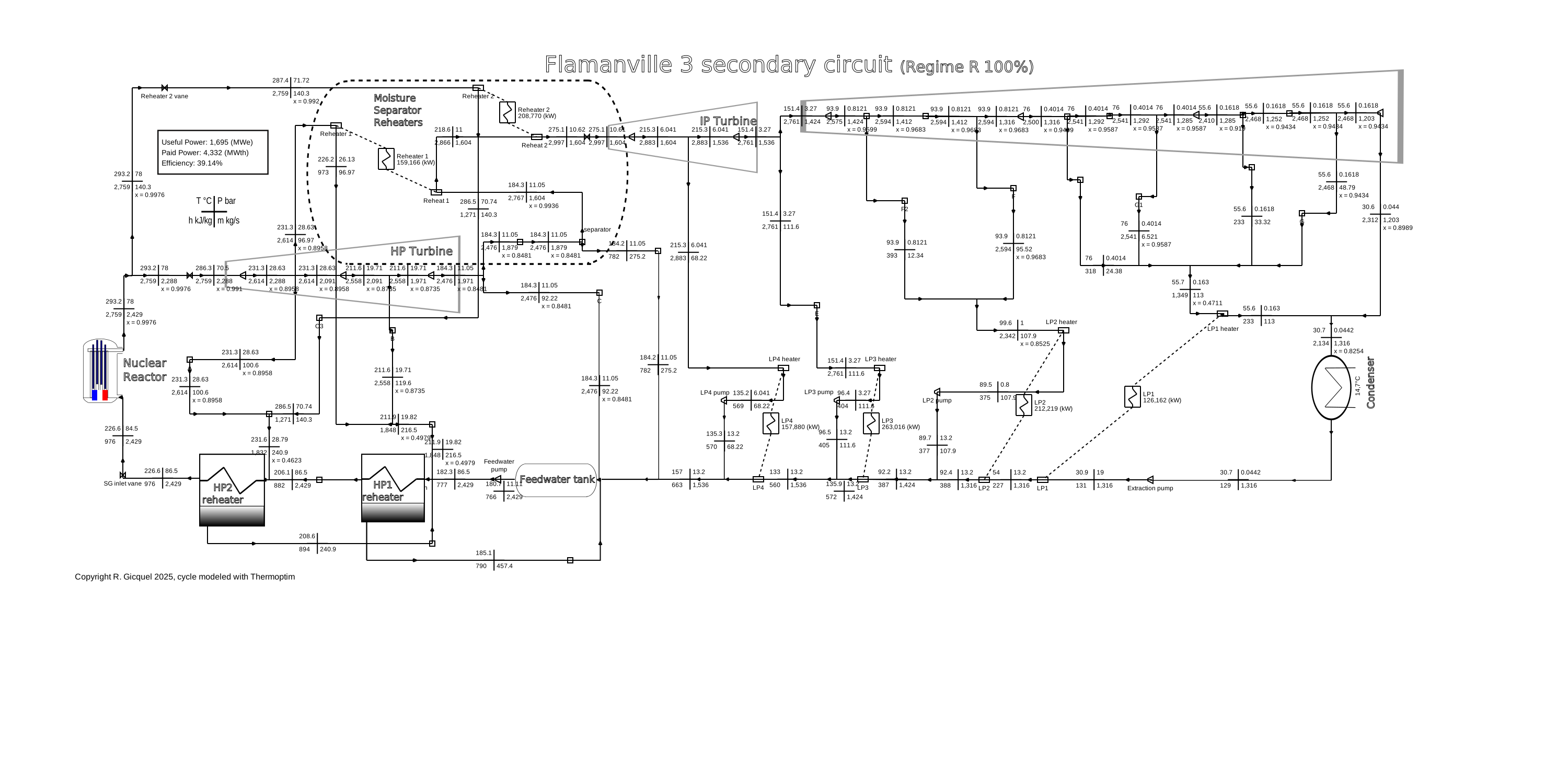
NUSCLE is designed to simulate part-load operation. It includes only four steam extractions and five turbine stage groups, compared to, for instance, eleven and nine respectively in the EPR Flamanville 3 cycle.
This compromise aims to serve educational purposes by offering an intermediate tool—somewhere between a full industrial model and an overly simplistic one.
Once validated, NUSCLE will be released as open-source, along with its complete Java code, to encourage reuse, deeper understanding, and further development.
As an educational tool, NUSCLE is not intended to deliver results as accurate as those produced by industrial-grade models. It has not yet undergone systematic testing and may still contain errors. However, we believe that sharing this current version is a valuable step forward, and we are seeking feedback and suggestions from beta testers (info@thermoptim.org).
NUSCLE enables users to:
Explore how key parameters affect the performance of various WCR types
Analyze part-load behavior of these cycles
Compare different reactor cycles
Access and understand the full set of equations, with the possibility to modify them as desired
Input Data
The part-load modeling of the EPR Flamanville 3 thermodynamic cycle is based on detailed official data provided by EDF to the French Nuclear Safety Authority (ASN) for licensing approval. This is a Generation III PWR, designed with significantly improved safety standards.
The data come from the knowledge models used by the plant’s designer and operator for system design and operation. As such, they can be considered highly reliable, pending availability of operational data—which will take several years, and may not be made publicly available.
These datasets constitute a rare and high-quality educational resource. The insights they provide are applicable not only to the EPR but also to a broad range of steam-based thermodynamic cycles used in water-cooled nuclear reactors. They may be particularly helpful for improving the modeling of Small Modular Reactors (SMRs) currently under development.
They also helped validate several empirical correlations implemented in NUSCLE.
Brief Overview of NUSCLE
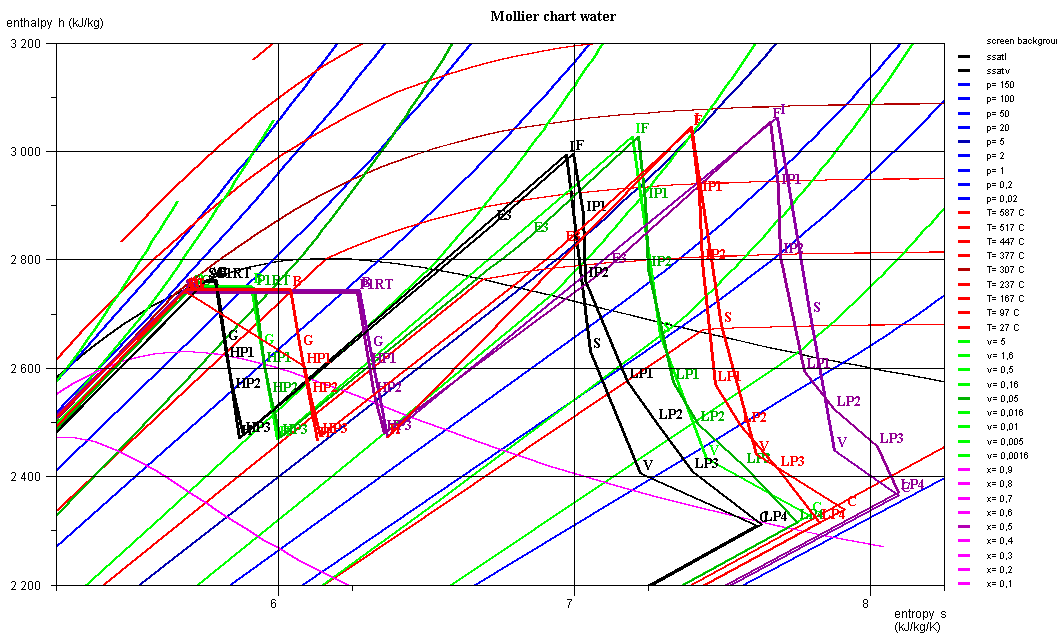
The two figures below illustrate the schematic generated of a 1680 MW EPR, as well as the simulated cycles plotted in the Mollier chart for power levels of 30%, 50%, 70%, and 100%.
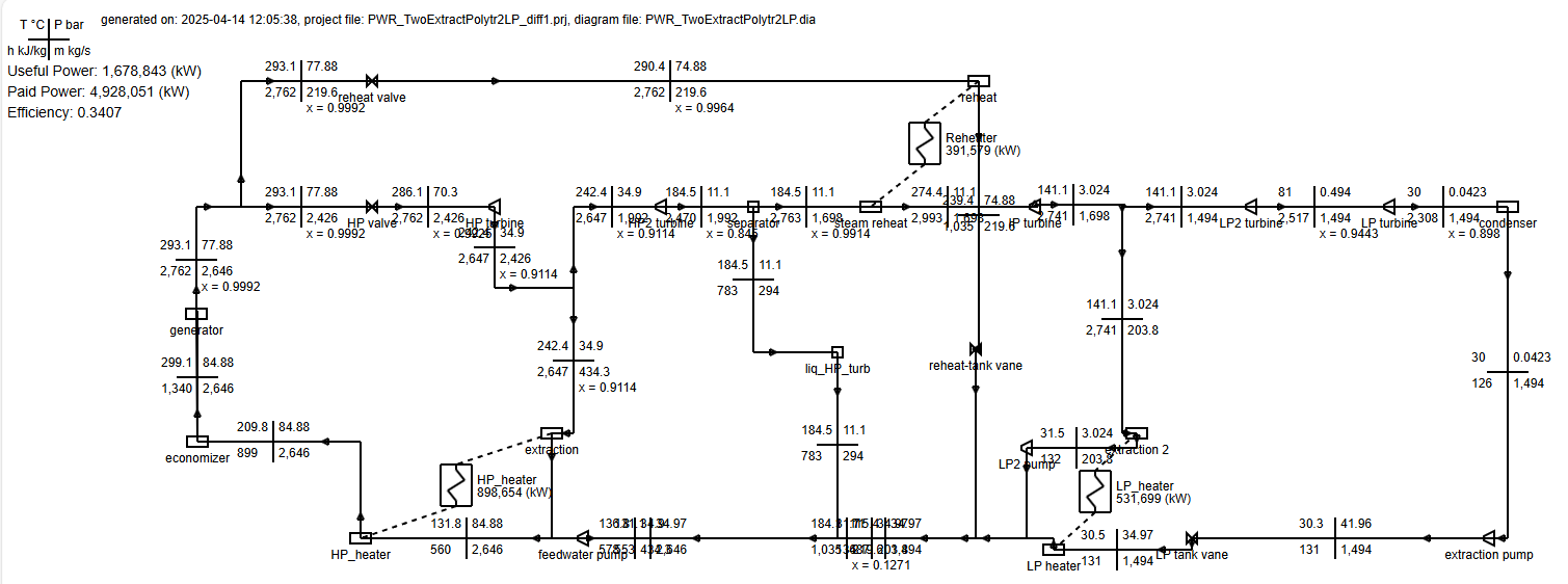
Although the model remains simplified—particularly regarding the feedwater system—it successfully reproduces the general trends of the EPR Flamanville 3 cycle. The simulation curves closely match the real ones for the HP and IP turbines. Discrepancies in the LP expansion line arise because the simplified model includes only two stage groups instead of the real system's more detailed layout.
A complete cycle model is available here:
👉 https://www.s4e2.com/download/diag/Flamanville_100_R_ASN_diff.svg
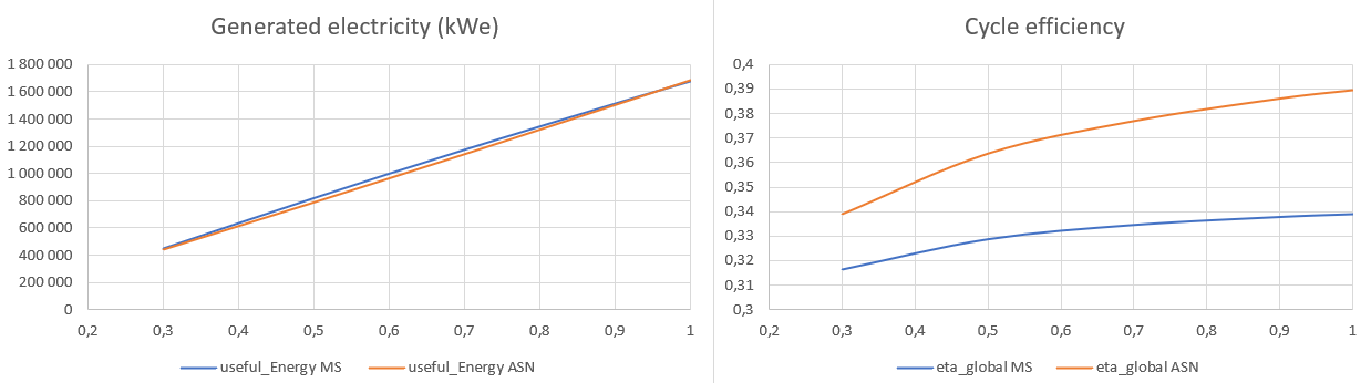
The global performance comparison chart below contrasts the ASN data with NUSCLE results. Generated power is accurately reproduced, but the cycle efficiency is lower in the simplified model. This is expected: NUSCLE includes only four steam extractions, versus eleven in the actual EPR cycle.
To match the real feedwater reheat temperature, the last extraction flow must be significantly increased. This in turn reduces the steam flow through the remaining turbine stages, which requires an increase in reactor mass flow rate, and thus, a higher thermal input to maintain power output—explaining the lower efficiency.
 ### User Interface
The main NUSCLE window is shown below.
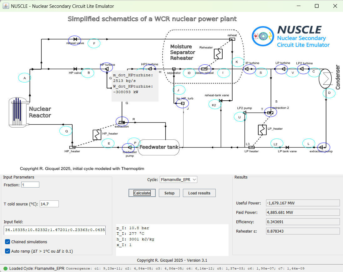
In the lower section of the screen, the following elements appear:
On the left:
Input fields for:
A fraction of the nominal power, presumably a positive number between 0 and 1. If the entered fraction is below 0.05, it is automatically set to this minimum value.
The cold source temperature. Both values must be entered using a dot (.) as the decimal separator.
Below these fields:
An "Input field" for entering additional data.
Two checkboxes:
"Chained simulations": Enables sequential simulations by reusing previously calculated results.
"Auto ramp (ΔT > 1°C or Δf ≥ 0.1)": Activates a gradual ramp of values for new simulations that deviate from initial conditions.
In the center:
A cycle selection dropdown menu, accompanied by three buttons and a text area for displaying values:
"Calculate": Initiates the computation.
"Setup": Determines the Stodola constants corresponding to the pressures entered in the aforementioned "Input field."
"Load Results": Loads a previous results file to resume from a prior state.
The text area displays relevant values during operations.
On the right:
The key performance indicators and their current values.
Results Window
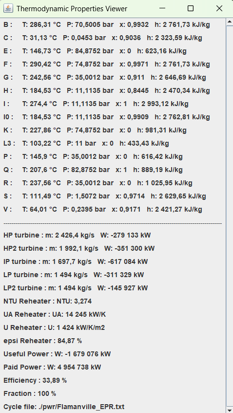
Each simulation generates a summary displayed in a separate window. The example shown corresponds to full load (fraction = 1).
Simultaneously, the full results are written to a text file named SimulResultsN.txt in the "res" directory. The counter N is reset each time the application launches and increments with every simulation, ensuring all results are traceable and preserved.
Finally, the expansion line plot is displayed in a third window using the Mollier diagram.
As shown in the figure, this window supports superimposing multiple plots, enabling users to:
Compare different cycles, or
Visualize how a cycle evolves as its parameters change.
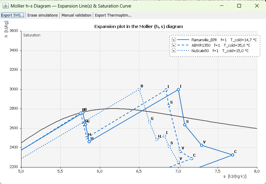
Clicking on one of the cycle identifiers in the legend (located in the top-right corner of the screen) toggles the visibility of the corresponding curve—hiding or displaying it.
This window provides four menu options to:
Export the displayed curves in SVG format (for high-quality vector graphics).
Clear all simulations currently shown in the window.
Manually validate or reject the display of a cycle after its calculation (e.g., to filter out incorrect or irrelevant results).
Export the cycle’s data points in Thermoptim’s cycle format, enabling compatibility with Thermoptim’s diagrams and full access to their features (e.g., further analysis, comparisons, or simulations).
Modifying Model Parameters
Two categories of parameters can be modified:
Simulation parameters, such as the fraction of the plant’s nominal capacity and the temperature of the cold source. These are defined in the main window of the simulator and are directly accessible to users for running their simulations.
Plant characterization parameters, defined in a configuration file (e.g., Flamanville_EPR.txt). These are intended primarily for instructors or advanced users, as selecting appropriate values requires a solid understanding of the underlying physical model.
When launched, NUSCLE loads a file called cycles.txt, which lists the available parameter sets. This list is used to populate the cycle selection menu.
Each configuration file can be edited either in a plain text editor or using the NUSCLE Parameters Viewer, a utility offering a more user-friendly interface.
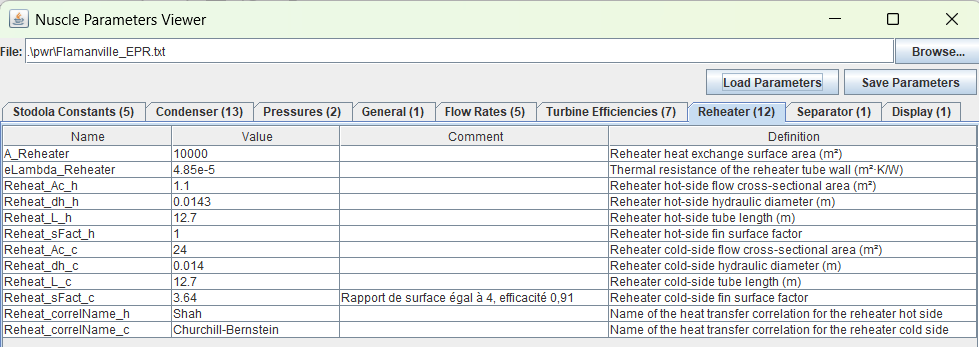
As shown in the following figure, parameters are grouped into nine categories. For each category, a list displays the parameter name, its value, any optional comments, and a description. Parameter editing is discussed in more detail later.
Solving Algorithm
The model uses two main inputs:
The load fraction (i.e., the fraction of the plant’s nominal power),
The cooling water temperature at the condenser inlet.
Given these inputs, the model solves for seven main unknowns:
The condensation pressure, determined by the condenser’s equilibrium,
The five inlet pressures for the turbine stage groups,
The outlet temperature of the high-temperature superheater.
These variables are considered “main” because all other model quantities are derived from them.
Solving the model involves a numerical algorithm capable of handling several hundred strongly nonlinear equations. This presents a number of challenges:
A valid set of initial guesses is crucial; otherwise, the solver may fail to converge or return unphysical results. We'll return to this issue later.
Using NUSCLE
To run the model, simply double-click the Nuscle_Simulator.jar file. The main interface appears.
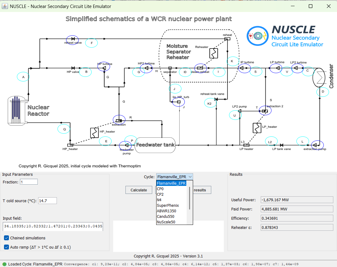
Select a cycle from the dropdown list.
The associated parameter file is loaded.
By default, the “Chained simulations” option is enabled, and the five turbine pressures are displayed in the “Input field”. These values come from the configuration file and can be edited. They will be used as initialization values for the solver.
If you do not want to use these values, uncheck “Chained simulations”. The solver will then use estimated pressure values derived from the Stodola constants.
“Setup” Button
A second button, “Setup”, appears to the right of “Calculate”.
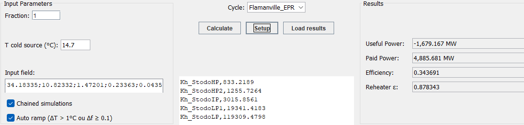
This button estimates the Stodola constants based on five pressure values entered in the input field (separated by ; and using . as the decimal separator).
Since turbine performance is modeled using Stodola’s law for each stage group, the intermediate pressure values must be consistent with the selected constants.
You can either:
Enter known Stodola constants in the parameter file and let the solver do its job, or
Use the setup mode, where you provide the desired intermediate pressures and let the algorithm compute the corresponding constants.
To activate this mode, set displaySetup = true in the configuration file.
When enabled, the “Setup” button becomes visible. To calculate the constants:
Enter the five intermediate pressures, followed by the condensation pressure, in descending order, separated by ;
Click “Setup”
The estimated constants will appear in the result field below the buttons, formatted for the parameter file. Simply copy them into the configuration file to make them available for future runs.
« Chained simulations » Option
The primary purpose of Chained simulations is to allow a sequence of runs starting from the previous result, while still allowing parameter adjustments between simulations.
As mentioned earlier, most simulation results are saved in files named simulResultsN.txt in the res folder, with N incremented between runs to facilitate post-processing.
Editing Parameters
As noted, there are two types of editable parameters:
Simulation parameters (power fraction, cold source temperature, and optionally initial pressure guesses), defined in the simulator’s main window and directly editable by users.
Plant-specific parameters, defined in a file named after the selected cycle (e.g., Flamanville_EPR.txt).
While the model is calibrated using part-load operating data from Flamanville 3 (EPR), it has broader applicability, and can be used to study other water-cooled reactors, including PWRs, BWRs, RBMKs, and CANDUs.
When NUSCLE starts, it loads a default configuration file from the pwr folder. This file contains a list of parameters defined over three comma-separated fields:
Parameter name,
Value,
Optional comment.
The figure below shows the part of the Flamanville_EPR.txt file related to the superheater configuration as it appears in a text editor.
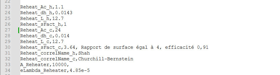
If a parameter appears on multiple lines, only the last one is used. This feature lets users keep several versions in the same file, with the active one placed at the end.
This allows you to keep several settings in the file either while waiting to find the best one, or to be able to come back to it later. All you have to do is copy the new configuration after the one that was in force until then
The NUSCLE Parameters Viewer displays parameters in the same structure.
It contains the values of the warmer parameters that we saw earlier in the text editor.
When you click “Save parameters”, the new values are appended to the configuration file.
⚠️ Since repeated saves grow the file quickly, we recommend removing outdated entries if no longer needed.
⚠️ Also, ensure that all parameter values are mutually consistent. Otherwise, results may be incorrect, or the model may fail to converge.
The configuration file is reloaded either when you select the cycle again from the dropdown menu, or when starting a new simulation with Chained simulations enabled.
This lets you observe how varying one or more parameters influences the results, by applying small, reasonable changes from one run to the next.
Starting from version 2.1 of Nuscle, it is possible to impose an initial degree of superheat on the model, in order to represent certain cycles that use it, by setting its value using the parameter dTsat_A, which appears in the 'Others' category of the utility.
Ensuring Proper Initialization
We refer to reasonable variations because, as previously noted, you may encounter convergence issues with the algorithm if the modifications are too large or if the initial variables are too far from the actual solution. To mitigate this, we have implemented a ramping system to help the algorithm converge, but this is not always sufficient.
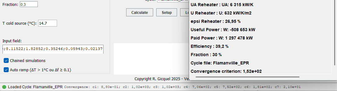
Convergence criteria are displayed at the bottom of the main window for each residual, and a global convergence criterion is shown at the bottom of the results window.
Three possible outcomes may occur:
1. NUSCLE converges, but with poor accuracy. We ran a simulation with a nominal power fraction set to 0.3, but the resulting convergence criteria are exceptionally high: 152 globally, with detailed residual values displayed at the bottom of the screen.
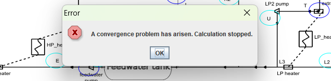
2 NUSCLE fails to find a solution, and you get an error message.
3 Nothing happens, indicating a severe failure.
In such cases, you have two options:
3.1 Restart NUSCLE, or witch to another cycle, then return to the one you were working on.
This resets the state for a clean start.
3.2 You can also look through previously saved result files (simulResultsN.txt) to find a run that successfully converged, and use its values as your new starting point.
Each file ends with two lines:
One with the turbine inlet pressures,
One with the convergence criteria.
Here is an example of unsuccessful convergence.

And here is one where the convergence has been successful:

By looking at your results from previous simulations in this way, you can go back to the last one that converged correctly.
Once you find a successful run, simply copy the pressures from the second-to-last line into the “Input field”, and run a new simulation with a nearby parameter set, keeping Chained simulations enabled.
By proceeding step by step, NUSCLE is more likely to converge successfully.
Post-Processing Simulation Results
You can post-process simulation outputs by copying them into a spreadsheet.
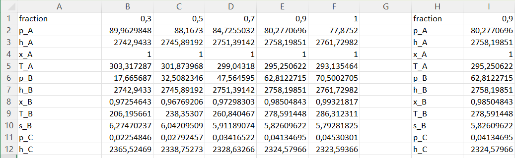
Here’s how:
Reserve two columns (e.g., H and I) for the simulation outputs,
Paste the labels in column A,
Paste each result set into subsequent columns.
This allows you to:
Perform custom calculations, or
Create graphs illustrating how key variables evolve across different simulation cases.
New Cycles Modeled in NUSCLE, Nuclear Secondary Circuit Lite Emulator
New cycles have been added to the list of those available in NUSCLE.
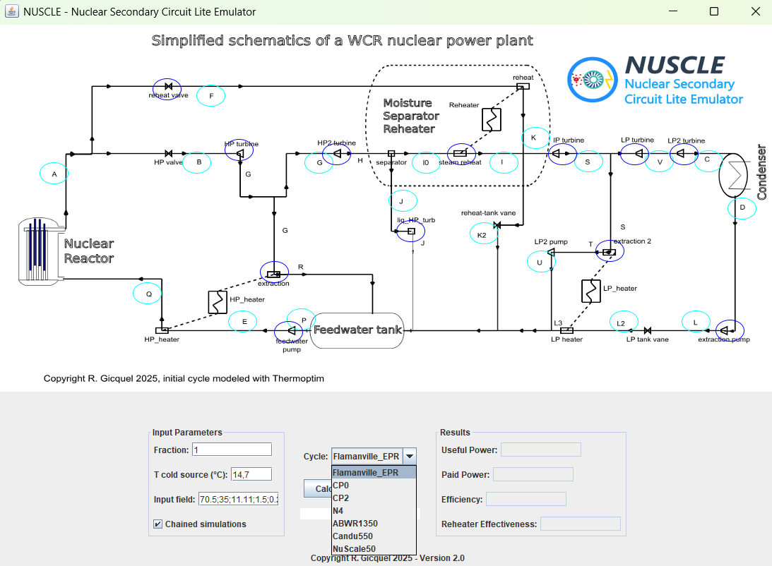
The list of available cycles now includes:
EPR Flamanville 3 (1650 MW), simplified NUSCLE cycle and full cycle, for 30%, 50%, 70%, 90%, and 100% of nominal power
French PWR plants: CP0 and CP2 (900 MW), N4 (1450 MW)
Hitachi ABWR plant (1350 MW)
Pickering CANDU plant (550 MW)
NuScale SMR (50 MW)
All files can still be downloaded at the following address:
http://www.s4e2.com/nuscle/Nuscle_diff.zip
#Flamanville #PWR #BWR #CP0 #CP2 #N4 #ABWR #Candu #NuScale
The NUSCLE models are simplified, but the plots in the thermodynamic charts correspond to detailed models for the three new cycles:
Mollier (h-s) chart:
https://s4e2.com/diag/fla3/HS-cycles-plotter.html
• Enthalpy (h-P) chart:
https://s4e2.com/diag/fla3/HP-cycles-plotter.html
• Entropy (T-s) chart:
https://s4e2.com/diag/fla3/TS-cycles-plotter.html
#Flamanville #PWR #BWR #CP0 #CP2 #N4 #ABWR #Candu #NuScale
Release of version 2.1 of NUSCLE
A number of improvements have been made to NUSCLE, particularly the ability to model secondary cycles with an initial superheat in order to represent SMRs such as NuScale.
Version 2.1 incorporates these changes.
All files can still be downloaded at the following address:
Release of NUSCLE Version 3.1
NUSCLE 3 is now available, packed with exciting new features, including:
Visualization of expansion lines in a Mollier diagram, allowing users to compare results from multiple simulations.
Export capabilities for cycles in a format compatible with Thermoptim’s interactive diagrams, as well as SVG format for high-quality vector graphics.
Ramping functionality to improve algorithm convergence when dealing with significant parameter variations.
Support for loading previous result files, enabling users to resume simulations from earlier states.
About NUSCLE NUSCLE (Nuclear Secondary Circuit Lite Emulator) is a simplified model of thermodynamic cycles coupled with water-cooled nuclear reactors, designed primarily for educational purposes. It includes:
Four extraction points,
Five distinct turbine stage groups,
A steam reheater and condenser, all modeled under off-design conditions.
Download NUSCLE 3.1 here:
http://www.s4e2.com/nuscle/Nuscle_diff.zip
#Flamanville #PWR #BWR #CP0 #CP2 #N4 #ABWR #Candu #NuScale