🛠️ Using Exergy Balances in Practice
Now that the conceptual foundations are in place, this page shows how exergy balances are actually used — and what precautions to take when interpreting them. Three questions are addressed in turn: how to optimise a cycle step by step, how the choice of source temperature Tk affects the results, and how two reactors with very similar energy efficiencies can have very different exergy profiles.
U1 — Reading a Balance to Guide Optimisation
An energy balance tells you how much energy is lost. An exergy balance tells you where, how much, and in what order to act. This is a fundamental difference for the engineer.
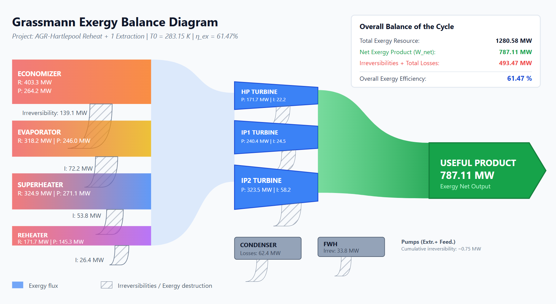
The example below follows four successive configurations of a steam cycle based on the AGR design (CO₂ gas coolant, Tk = 700 °C, T₀ = 20 °C). Each configuration was chosen by reading the balance from the previous step.
The four configurations
The exergy balance files are accessible through the links in this table.
| Configuration | η Xh | η energy | Dominant irreversibility |
|---|---|---|---|
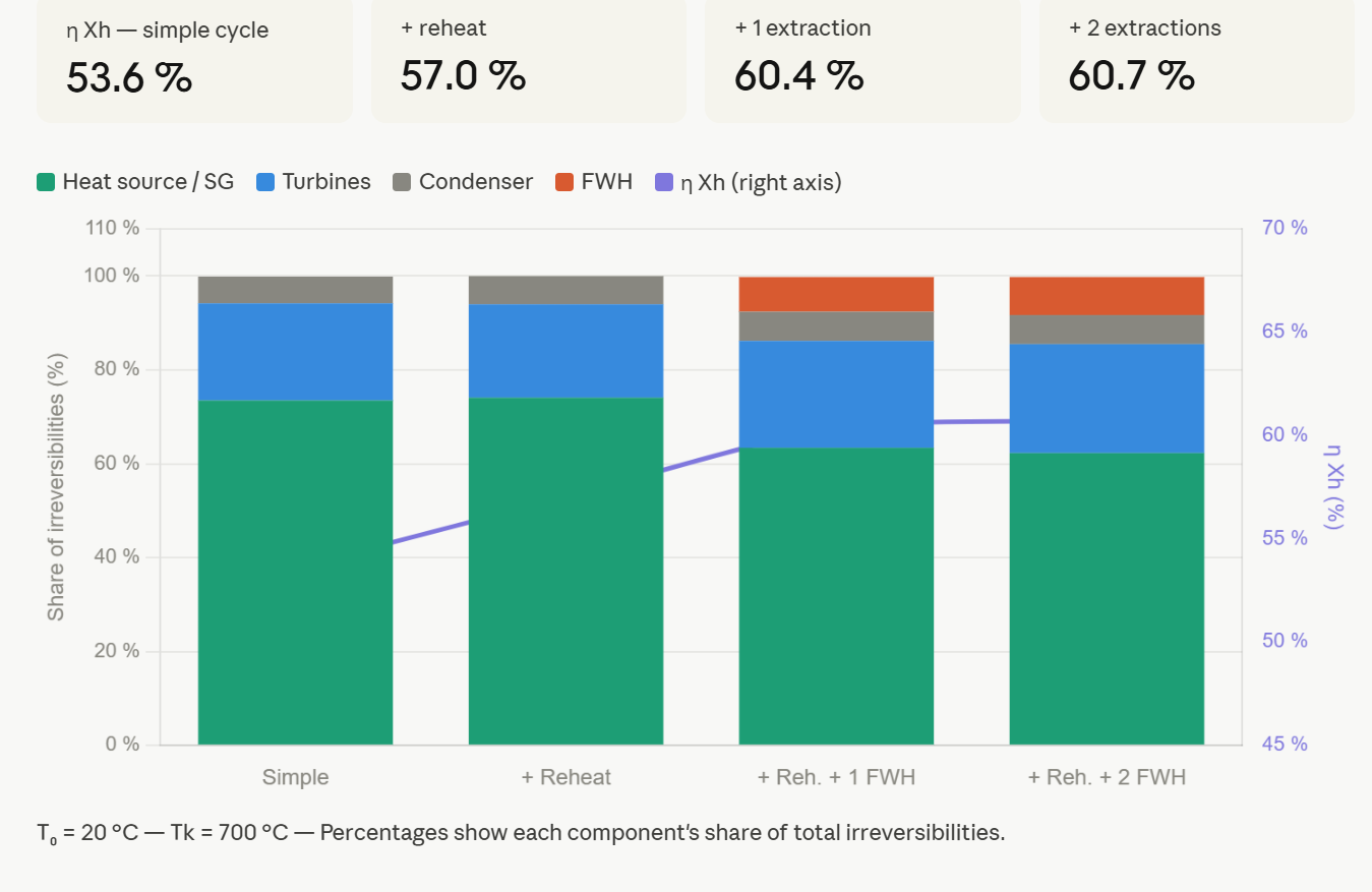
| Simple cycle | 53.6 % | 37.5 % | Source / SG: 73.5 % |
| + Reheat | 57.0 % | 39.9 % | Source / SG: 74.1 % |
| + Reheat + 1 FWH | 60.4 % | 42.2 % | Source / SG: 63.4 % — FWH: 7.4 % |
| + Reheat + 2 FWH | 60.7 % | 42.4 % | Source / SG: 62.3 % — FWH: 8.1 % |
What is striking is the evolution of the overall exergy efficiency as technological modifications take place.
Step-by-step reasoning
Simple cycle — η Xh = 53.6 %
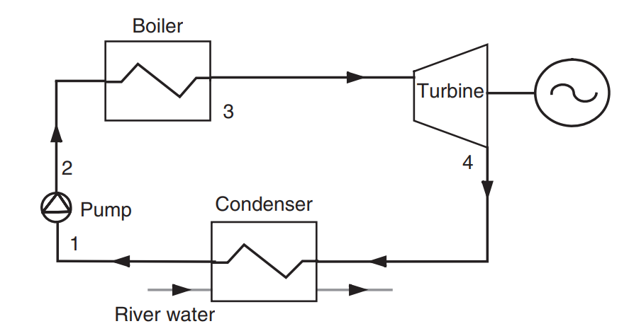
The balance is immediately readable: the source (steam generator) accounts for 73.5 % of total irreversibilities. The economiser alone absorbs 49 %. Turbines represent only 20.7 %, the condenser 5.7 %. The message is unambiguous: the main lever is not in the turbines — it is in the heat transfer from the gas to the steam.
+ Reheat — η Xh = 57.0 % (+3.4 pts)
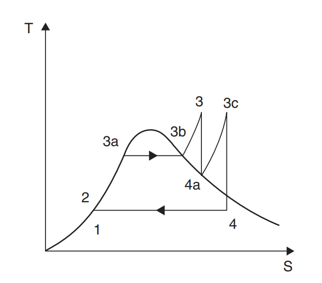
In a cycle with reheats, we begin by partially expanding the steam, then it passes again into the boiler, where it is heated at the new pressure to approximately the maximum cycle temperature.
This results in efficiency gains of a few percent and, most importantly, as shown in the diagram, increased quality at the end of expansion, which is always beneficial for extending the life of turbine blades.
Reheat redistributes some of the SG heat through an additional turbine stage and improves mean isentropic efficiency. Yet the source remains dominant at 74.1 % — its relative weight has barely changed. A different lever is needed.
+ 1 feedwater extraction (FWH) — η Xh = 60.4 % (+3.4 pts)
In a steam cycle, it is possible to undertake partial regeneration by using part of the heat rejected during expansion for preheating the pressurized liquid water before it enters the boiler.
Consider a cycle with reheat. If we extract a small quantity of steam, called extraction steam or bleed steam, at the outlet of the first expansion, at point 4a in the figure, its pressure remains high enough to condense it at a temperature that allows preheating the pressurized water leaving the pump at point 2.
The enthalpy of the vapor is much greater than that of the liquid, due to the latent heat of vaporization. It is then possible to preheat the liquid using a small extraction of steam during expansion.
This operation is carried out in specific components called feedwater reheaters FWH.
This cycle is called a regenerative Rankine cycle, also known as an extraction and reheat steam cycle.
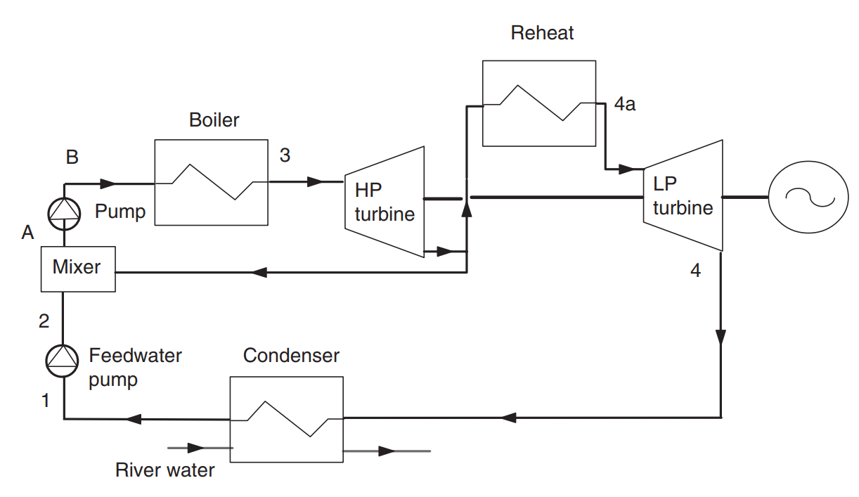
Now the source falls to 63.4 % (−10.7 pts). Preheating the feedwater reduces the temperature gap in the economiser, which had been the dominant component since the start. The FWH carries its own irreversibility cost (7.4 %) but saves far more on the source.
+ 2nd extraction — η Xh = 60.7 % (+0.3 pts only)
The source falls slightly again (62.3 %), but the marginal gain collapses. The balance signals that diminishing returns have been reached: the second extraction costs almost as much as it saves.
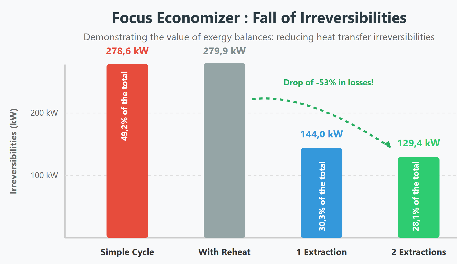
Steam extraction allows the feedwater to be preheated (via the FWH) before it enters the economizer. By reducing the temperature difference in the economizer, exergy analysis shows that its irreversibilities have been halved (from 278.5 kW to 129.4 kW).
The lesson: at each step, the exergy balance indicated which lever to pull by tracking the dominant component. It serves as a guide for optimization.
U2 — The Source Temperature Convention: the Choice That Changes Everything
All the balances in this section use a source temperature Tk chosen according to the type of heat exchange between the coolant and the steam. The convention is:
| Exchange type | ΔT | Rationale |
|---|---|---|
| Liquid coolant → boiling (WCR) | +35 °C | Typical pinch for liquid/boiling exchange |
| Liquid sodium → steam (SFR) | +50 °C | Larger pinch for liquid/vapour exchange |
| Supercritical water → steam (SCWR) | +50 °C | Same |
| Gas → steam (AGR, HTR) | +60 °C | Larger pinch for gas/vapour exchange |
This convention has a direct consequence: a higher Tk mechanically reduces η Xh, because more of the core irreversibilities are attributed to the source component. Two reactors cannot be compared on η Xh alone without knowing their respective Tk values.
A concrete illustration — what happens when Tk increases on the Flamanville EPR:
The ExergyTkSensitivity tool sweeps Tk from the balance value to 1000 °C, keeping T₀ and all other irreversibilities fixed. Applied to the EPR Flamanville detailed balance (Tk = 334 °C, T₀ = 15 °C):
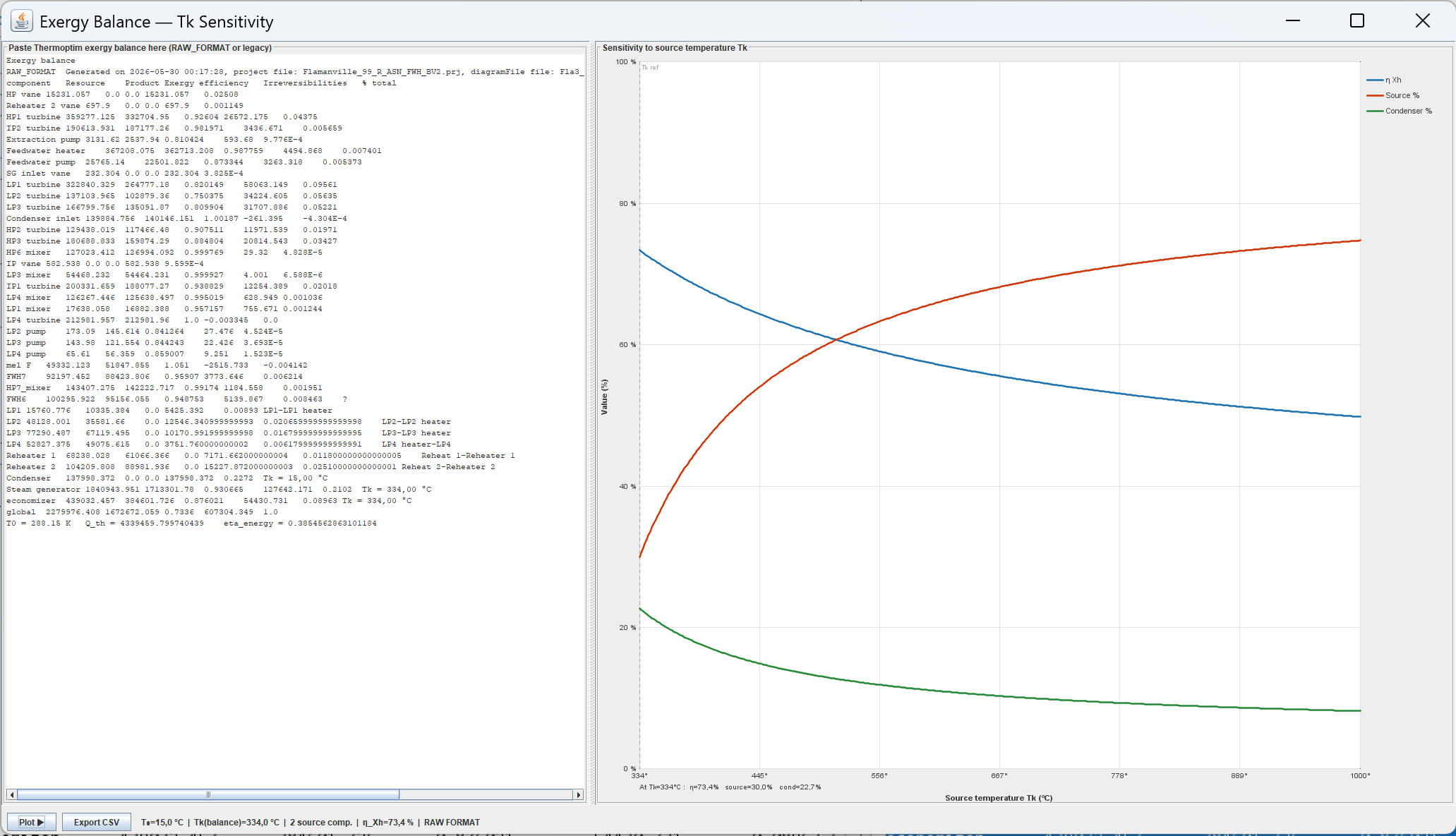 Sensitivity of η Xh (blue), source % (red) and condenser % (green) to source temperature Tk for the EPR Flamanville detailed model.
- At Tk = 334 °C (reference): η Xh = 73.4 %, source = 30.0 %, condenser = 22.7 %
- At Tk ≈ 445 °C: source and condenser curves cross (~30 % each) — the source becomes dominant
- At Tk = 700 °C: η Xh ≈ 54 %, source ≈ 49 %, condenser ≈ 12 %
- At Tk = 1000 °C: η Xh ≈ 35 %, source ≈ 57 %, condenser ≈ 9 %
The cycle has not changed. Only the accounting of the source has changed. This is why the AGR (Tk = 699 °C, η Xh = 61.8 %) and the EPR (Tk = 334 °C, η Xh = 73.9 %) cannot be compared directly: the AGR balance includes the irreversibilities of the entire CO₂ coolant circuit, while the EPR balance only includes the near-boiling heat exchange at 334 °C.
The crossing point at ~445 °C is particularly informative: below this temperature, the condenser is the larger structural loss term; above it, the source dominates.
The physical basis: Carnot factors and what Tk really controls
The source temperature Tk enters the exergy balance through the Carnot factor (1 − T₀/Tk), which converts a heat flow Q into its exergy equivalent:
Xh = Q × (1 − T₀/Tk)
Changing Tk therefore changes the exergy attributed to a heat exchange — and this has very different consequences depending on whether it is the hot source or the cold source that is varied.
Varying the hot source temperature Tk affects only the components that exchange heat with the hot source — typically the steam generator, economiser, core, or IHX. All other irreversibilities in the balance (turbines, feedwater heaters, mixing valves, pumps) are computed from fluid state differences and do not depend on Tk. This is exactly what the ExergyTkSensitivity tool exploits: it sweeps Tk over a range and recomputes only the source component contributions, keeping everything else fixed. The result is a clean sensitivity curve that answers the question “how much of the η Xh difference between two reactors is due to the Tk convention?”
It is precisely because the thermal power Q transferred by the hot source can be back-calculated from the source exergy and Tk — via Q = Xh_source / (1 − T₀/Tk) — that the values Q_th and η energy have been appended to the bottom of the exergy balance files. Knowing Q_th allows the energy efficiency to be derived directly from the balance, without requiring a separate energy model. The ExerBalanceHX post-processing tool computes and writes these two values automatically when it processes a balance.
Varying the cold source temperature Tcond is an entirely different matter. Tcond is the temperature of the condenser cooling fluid. If it changes, the condenser thermal equilibrium shifts, its condensation pressure changes, and — through the turbine expansion ratios — the pressures and enthalpies at every turbine stage are modified. The irreversibilities of all turbine stages change, the extraction flows to the feedwater heaters change, and the entire cycle operates at a new off-design point. This cannot be studied by a simple balance recalculation: it requires a full thermodynamic cycle model operating at the new conditions.
This is one of the specific strengths of Nuscle: because it models the complete secondary circuit thermodynamically, it can simulate the effect of a change in condensation temperature and generate a new consistent exergy balance for the modified operating point — something that a post-processing tool like ExergyTkSensitivity cannot do. The NuScale US460 and ABWR cases (both designed with air-cooled condensers at 35 °C rather than the standard 15 °C) will be studied this way when the corresponding Nuscle parametric models are available.
Two valid questions, two valid conventions:
- “How good is the secondary cycle alone?” → Use a Tk close to the actual heat exchange temperature (Tprimary + ΔT). Differences between reactors reflect cycle quality.
- “How efficiently does the full plant convert nuclear heat?” → Use a common Tk for all reactors. Differences reflect the combination of core and cycle performance.
Both are legitimate. The key is to state which question is being answered before presenting the numbers.
U3 — Exergy Balances as a Diagnostic Instrument
The AGR four-step example in U1 illustrates a general principle: as a cycle approaches its thermodynamic optimum, the dominant irreversibility shifts from the source to the components that are harder to reduce.
The EPR Flamanville 3 is a 1 650 MWe pressurised water reactor, primary at 300 °C / 155 bar, steam at 294 °C / 75 bar, with eight feedwater heaters, double reheat, and six LP turbine stages. It is the most powerful reactor currently operating in France.
For the EPR Flamanville detailed model (η Xh = 73.9 %), the exergy balance shows:
| Component | % of total irreversibilities |
|---|---|
| Source (SG + economiser) | 30.0 % |
| Turbines | 32.2 % |
| Condenser | 22.7 % |
| Feedwater heaters (FWH) | 0.7 % |
| Reheaters | 3.8 % |
| Remaining | 10.6 % |
No single component dominates. The balance is well distributed — a signature of a well-optimised cycle. Any further improvement would require acting on multiple components simultaneously for marginal gains.
The VVER-70 is the first Soviet pressurised water reactor design, installed at the Novovoronezh plant (units 1–2, 1964–1969). Three K-70-29 turbines of 70 MWe each give a total output of 210 MWe from a thermal power of 760 MWth. The primary coolant operates at approximately 248 °C, steam is produced at 29 bar — saturated, with no superheat. Between the HP and LP turbine sections, a moisture separator reduces liquid content to ~1 % but does not raise steam temperature.
For the VVER-70 (η Xh = 57.5 %, Nuscle model), the exergy balance shows:
| Component | % |
|---|---|
| Source | 39.5 % |
| Turbines | 36.6 % |
| Condenser | 19.2 % |
| FWH | 1.6 % |
Here the source is clearly dominant (39.5 %) and the FWH contribution is almost negligible (1.6 %). The balance immediately points to two actions: reduce the temperature gap in the steam generator (e.g., by adding superheat) and increase the regenerative feedwater heating. These are precisely the changes made in the VVER-1000, which achieves η Xh = 68.0 % — a gain of 10.5 points.
Two modelling notes for the VVER-70 are important for correct interpretation:
No reheat after the separator. The K-70-29 turbine uses a moisture separator only — there is no steam reheater between the HP and LP sections. The separator reduces liquid content to approximately 1 %, but without raising the steam temperature. The Nuscle model reflects this by setting the reheat flow to effectively zero; the corresponding lines have been removed from the published balance. This means the VVER-70 and VVER-1000 are not simply two generations of the same design — they represent two fundamentally different cycle philosophies (saturated steam + separator vs superheated steam + MSR).
Talim is estimated. The feedwater inlet temperature to the steam generator (Talim) is not documented in available sources for the Novovoronezh unit 1-2. It has been estimated from the known thermal power (760 MWth) and electrical output (210 MWe). A ±20 °C uncertainty on Talim propagates to approximately ±3 pts on the source % and FWH % individually, but affects η Xh global by less than ±0.5 pt. The η Xh = 57.5 % figure is therefore robust; the component breakdown carries a moderate uncertainty on the source/FWH split.
The exergy balance is a diagnostic instrument. It does not prescribe solutions, but it ranks the components by their contribution to total irreversibility — and that ranking is the starting point for any systematic optimisation effort.